Importing outputs into R

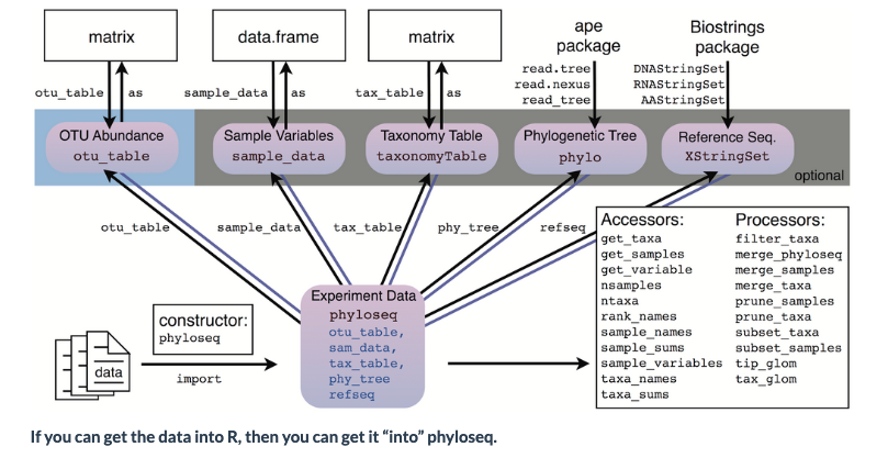
For examining the results of our analysis in R, we primarily be using the Phyloseq package, with some additional packages.

There are many possible file and data types that can be imported into Phyloseq:

alt_text

# load the packages
library('phyloseq')
library('tibble')
library('ggplot2')
library('dplyr')
library('tidyr')
library('ape')
library('vegan')
library('stringr')

# set the working directory
setwd('../plots')

Import the frequency table

import_table <- read.table('../otus/otu_frequency_table.tsv',header=TRUE,sep='\t',row.names=1, comment.char = "")

head(import_table)

A data.frame: 6 × 11
	AM1	AM2	AM3	AM4	AM5	AM6	AS2	AS3	AS4	AS5	AS6
	<int>	<int>	<int>	<int>	<int>	<int>	<int>	<int>	<int>	<int>	<int>
OTU.1	723	3634	0	2907	171	1956	2730	2856	4192	3797	3392
OTU.10	0	0	0	0	0	0	2223	0	0	1024	0
OTU.11	1892	0	0	0	82	113	0	0	0	0	0
OTU.12	0	1587	0	0	0	0	0	0	0	0	0
OTU.13	0	0	0	0	0	0	0	0	0	1472	0
OTU.14	0	0	0	0	0	0	0	0	0	0	1087

# convert to a matrix for Phyloseq
otumat <- as.matrix(import_table)
head(otumat)

A matrix: 6 × 11 of type int
	AM1	AM2	AM4	AM5	AM6	AS2	AS3	AS4	AS5	AS6
OTU.1	723	3634	2907	171	1956	2730	2856	4192	3797	3392
OTU.10	0	0	0	0	0	2223	0	0	1024	0
OTU.11	1892	0	0	82	113	0	0	0	0	0
OTU.12	0	1587	0	0	0	0	0	0	0	0
OTU.13	0	0	0	0	0	0	0	0	1472	0
OTU.14	0	0	0	0	0	0	0	0	0	1087

# create a Phyloseq object using the function `otu_table`
OTU = otu_table(otumat, taxa_are_rows = TRUE)
head(OTU)

A otu_table: 6 × 11 of type int
	AM1	AM2	AM4	AM5	AM6	AS2	AS3	AS4	AS5	AS6
OTU.1	723	3634	2907	171	1956	2730	2856	4192	3797	3392
OTU.10	0	0	0	0	0	2223	0	0	1024	0
OTU.11	1892	0	0	82	113	0	0	0	0	0
OTU.12	0	1587	0	0	0	0	0	0	0	0
OTU.13	0	0	0	0	0	0	0	0	1472	0
OTU.14	0	0	0	0	0	0	0	0	0	1087

import the taxonomy table (exported from Qiime2)

Now we will import the taxonomy table. After importing to R, we will have to split the taxonomy column into separate columns for each taxon, so that Phyloseq can recognise it.

import_taxa <- read.table('../taxonomy/otu_taxonomy.tsv',header=TRUE,sep='\t',row.names=1)
head(import_taxa)

A data.frame: 6 × 2
	Taxon	Confidence
	<chr>	<dbl>
OTU.1	d__Eukaryota;p__Chordata;c__Actinopteri;o__Scombriformes;f__Gempylidae;g__Thyrsites;s__Thyrsites_atun	1.0000000
OTU.2	d__Eukaryota;p__Chordata;c__Actinopteri;o__Mugiliformes;f__Mugilidae;g__Aldrichetta;s__Aldrichetta_forsteri	0.9999999
OTU.3	d__Eukaryota;p__Chordata;c__Actinopteri;o__Perciformes;f__Bovichtidae;g__Bovichtus;s__Bovichtus_variegatus	0.9999979
OTU.4	d__Eukaryota;p__Chordata;c__Actinopteri;o__Blenniiformes;f__Tripterygiidae;g__Forsterygion;s__Forsterygion_lapillum	1.0000000
OTU.5	d__Eukaryota;p__Chordata;c__Actinopteri;o__Labriformes;f__Labridae;g__Notolabrus;s__Notolabrus_fucicola	0.9996494
OTU.6	d__Eukaryota;p__Chordata;c__Actinopteri;o__Blenniiformes;f__Tripterygiidae;g__Forsterygion;s__Forsterygion_lapillum	1.0000000

You can see that the taxonomic lineage is in one column. We will run a pipe to split each taxonomic rank into separate columns, and also take out the Qiime-style title for each rank (e.g. ‘d__’). Finally, we will convert the data frame into a matrix so it is readable by Phyloseq.

# First we have to provide names for the new columns
ranks <- c("kingdom","phylum","class","order","family","genus","species")

taxonomy <- import_taxa %>%
  mutate_at('Taxon',str_replace_all, "[a-z]__","") %>%
  separate(Taxon, sep = ';', into=ranks,remove = TRUE) %>%
  as.matrix()
head(taxonomy)

Warning message:
“Expected 7 pieces. Missing pieces filled with `NA` in 13 rows [9, 13, 15, 17, 25, 26, 27, 28, 29, 30, 31, 32, 33].”

A matrix: 6 × 8 of type chr
	kingdom	phylum	class	order	family	genus	species	Confidence
OTU.1	Eukaryota	Chordata	Actinopteri	Scombriformes	Gempylidae	Thyrsites	Thyrsites_atun	1.0000000
OTU.2	Eukaryota	Chordata	Actinopteri	Mugiliformes	Mugilidae	Aldrichetta	Aldrichetta_forsteri	0.9999999
OTU.3	Eukaryota	Chordata	Actinopteri	Perciformes	Bovichtidae	Bovichtus	Bovichtus_variegatus	0.9999979
OTU.4	Eukaryota	Chordata	Actinopteri	Blenniiformes	Tripterygiidae	Forsterygion	Forsterygion_lapillum	1.0000000
OTU.5	Eukaryota	Chordata	Actinopteri	Labriformes	Labridae	Notolabrus	Notolabrus_fucicola	0.9996494
OTU.6	Eukaryota	Chordata	Actinopteri	Blenniiformes	Tripterygiidae	Forsterygion	Forsterygion_lapillum	1.0000000

# Create a taxonomy class object
TAX = tax_table(taxonomy)

Import the sample metadata

metadata <- read.table('../docs/sample_metadata.tsv',header = T,sep='\t',row.names = 1)
metadata

A data.frame: 12 × 8
	fwd_barcode	rev_barcode	forward_primer	reverse_primer	location	temperature	salinity	sample
	<chr>	<chr>	<chr>	<chr>	<chr>	<int>	<int>	<chr>
AM1	GAAGAG	TAGCGTCG	GACCCTATGGAGCTTTAGAC	CGCTGTTATCCCTADRGTAACT	mudflats	12	32	AM1
AM2	GAAGAG	TCTACTCG	GACCCTATGGAGCTTTAGAC	CGCTGTTATCCCTADRGTAACT	mudflats	14	32	AM2
AM3	GAAGAG	ATGACTCG	GACCCTATGGAGCTTTAGAC	CGCTGTTATCCCTADRGTAACT	mudflats	12	32	AM3
AM4	GAAGAG	ATCTATCG	GACCCTATGGAGCTTTAGAC	CGCTGTTATCCCTADRGTAACT	mudflats	10	32	AM4
AM5	GAAGAG	ACAGATCG	GACCCTATGGAGCTTTAGAC	CGCTGTTATCCCTADRGTAACT	mudflats	12	34	AM5
AM6	GAAGAG	ATACTGCG	GACCCTATGGAGCTTTAGAC	CGCTGTTATCCCTADRGTAACT	mudflats	10	34	AM6
AS2	GAAGAG	AGATACTC	GACCCTATGGAGCTTTAGAC	CGCTGTTATCCCTADRGTAACT	shore	12	32	AS2
AS3	GAAGAG	ATGCGATG	GACCCTATGGAGCTTTAGAC	CGCTGTTATCCCTADRGTAACT	shore	12	32	AS3
AS4	GAAGAG	TGCTACTC	GACCCTATGGAGCTTTAGAC	CGCTGTTATCCCTADRGTAACT	shore	10	34	AS4
AS5	GAAGAG	ACGTCATG	GACCCTATGGAGCTTTAGAC	CGCTGTTATCCCTADRGTAACT	shore	14	34	AS5
AS6	GAAGAG	TCATGTCG	GACCCTATGGAGCTTTAGAC	CGCTGTTATCCCTADRGTAACT	shore	10	34	AS6
ASN	GAAGAG	AGACGCTC	GACCCTATGGAGCTTTAGAC	CGCTGTTATCCCTADRGTAACT	negative	NA	NA	ASN

# As we are not using the negative control, we will remove it
metadata <- metadata[1:11,1:8]
tail(metadata)

A data.frame: 6 × 8
	fwd_barcode	rev_barcode	forward_primer	reverse_primer	location	temperature	salinity	sample
	<chr>	<chr>	<chr>	<chr>	<chr>	<int>	<int>	<chr>
AM6	GAAGAG	ATACTGCG	GACCCTATGGAGCTTTAGAC	CGCTGTTATCCCTADRGTAACT	mudflats	10	34	AM6
AS2	GAAGAG	AGATACTC	GACCCTATGGAGCTTTAGAC	CGCTGTTATCCCTADRGTAACT	shore	12	32	AS2
AS3	GAAGAG	ATGCGATG	GACCCTATGGAGCTTTAGAC	CGCTGTTATCCCTADRGTAACT	shore	12	32	AS3
AS4	GAAGAG	TGCTACTC	GACCCTATGGAGCTTTAGAC	CGCTGTTATCCCTADRGTAACT	shore	10	34	AS4
AS5	GAAGAG	ACGTCATG	GACCCTATGGAGCTTTAGAC	CGCTGTTATCCCTADRGTAACT	shore	14	34	AS5
AS6	GAAGAG	TCATGTCG	GACCCTATGGAGCTTTAGAC	CGCTGTTATCCCTADRGTAACT	shore	10	34	AS6

# Create a Phyloseq sample_data-class
META <- sample_data(metadata)

Import the phylogenetic tree

otu_tree <- read.tree(file='../otus/otu_rooted_tree.nwk')
otu_tree

Phylogenetic tree with 33 tips and 32 internal nodes.

Tip labels:
  OTU.33, OTU.8, OTU.21, OTU.29, OTU.17, OTU.16, ...
Node labels:
  root, , 0.870, 0.647, 0.637, 0.965, ...

Rooted; includes branch lengths.

## Let's have a look at the tree
plot(otu_tree)

png

Create a Phyloseq object

Now that we have all the components, it is time to create a Phyloseq object

pseq <- phyloseq(OTU,TAX,META,otu_tree)
pseq

phyloseq-class experiment-level object
otu_table()   OTU Table:         [ 33 taxa and 11 samples ]
sample_data() Sample Data:       [ 11 samples by 8 sample variables ]
tax_table()   Taxonomy Table:    [ 33 taxa by 8 taxonomic ranks ]
phy_tree()    Phylogenetic Tree: [ 33 tips and 32 internal nodes ]

Initial data inspection

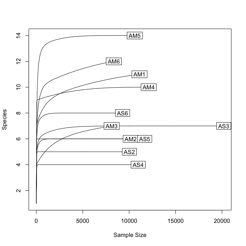
Now that we have our Phyloseq object, we will take a look at it. One of the first steps is to check alpha rarefaction of species richness. This is done to show that there has been sufficient sequencing to detect most species (OTUs).

# rarefaction
rarecurve(t(otu_table(pseq)), step=50, cex=1)

png

# create a bar plot of abundance
plot_bar(pseq)

png

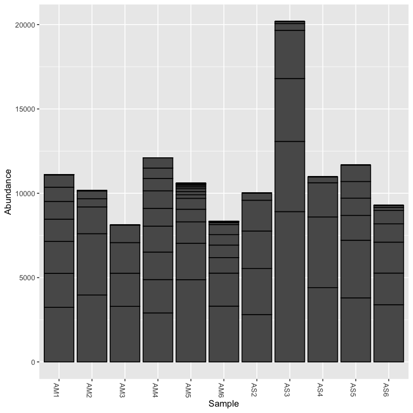
# some basic stats
print(min(sample_sums(pseq)))
print(max(sample_sums(pseq)))

[1] 8117
[1] 20184

Rarefy the data

From the initial look at the data, it is obvious that the sample AS3 has about twice as many reads as any of the other samples. We can use rarefaction to simulate an even number of reads per sample. Rarefying the data is preferred for some analyses, though there is some debate. We will create a rarefied version of the Phyloseq object.

# we will rarefy the data around 90% of the lowest sample
pseq.rarefied <- rarefy_even_depth(pseq, rngseed=1, sample.size=0.9*min(sample_sums(pseq)), replace=F)

`set.seed(1)` was used to initialize repeatable random subsampling.

Please record this for your records so others can reproduce.

Try `set.seed(1); .Random.seed` for the full vector

...

# now plot the rarefied version
plot_bar(pseq.rarefied)

png

Saving your work to files

You can save the Phyloseq object you just created, and then import it into another R session later. This way you do not have to re-import all the components separately.

Also, below are a couple of examples of saving graphs. There are many options for this that you can explore to create publication-quality graphics of your results

# save the phyloseq object
saveRDS(pseq, 'fish_phyloseq.rds')

# also save the rarefied version
saveRDS(pseq.rarefied, 'fish_phyloseq_rarefied.rds')

Saving a graph to file

# open a pdf file
pdf('species_richness_plot.pdf')
# run the plot, or add the saved one
rarecurve(t(otu_table(pseq)), step=50, cex=1.5, col='blue',lty=2)
# close the pdf
dev.off()

pdf: 2

# there are other graphic formats that you can use
jpeg("species_richness_plot.jpg", width = 800, height = 800)
rarecurve(t(otu_table(pseq)), step=50, cex=1.5, col='blue',lty=2)
dev.off()

pdf: 2